Animating MCMC in Julia

Introduction

One of my favorite aspects about Julia is how simple it is to build really high quality graphs and plots. I have used base plotting and {ggplot2} in R as well as matplotlib in python for several years. Those packages are great, and I think Plots.jl has a place among them. It has several cool features out of the box that are super easy to use, and boasts a “time to first (beautiful) plot” that is competitive. As the Julia data science community continues to grow, several other plotting libraries have emerged such as makie.jl and Algebra of Graphics. I have yet to dive into those, but as with everything in Julia, they look super cool!

In this post I will demonstrate the power of Plots.jl by making an animation of an MCMC sampler exploring the posterior distribuiton of a simple Normal-Normal model.

Imports

For this, we will need to load in several packages for stats, plotting, and performing the MCMC sampling. We will use the Turing.jl library to define our Bayesian model.

using Random, StatsBase , KernelDensity # for stats
using Plots, StatsPlots # for plots
using Distributions, Turing # for MCMC

Simulated Data

We need some data to fit our model. For this, we will simulate 100 observations from a normal distribution with mean 4 and standard deviation of 2.

# Define Normal Distribution
mu_true = 4;
sd_true = 2;
dist = Normal(mu_true, sd_true);

# Sample from the distribution
N = 100;
Random.seed!(1234);
data = rand(dist, N);

Defining and Sampling the Model

The next thing we need is a model. In Turing.jl this is extremely simple to do. We simply define our priors and the likelihood distribution and we are good to go!

For this model, we are using a (considerably) uniformative Normal(0,5) prior for μ and an Exponential(1) prior for σ.

# Define Turing Model
@model function normal_model(y)
	# Priors
	μ ~ Normal(0,5)
	σ ~ Exponential(1)

	# Likelihood
	J = length(y)
	for i in 1:J
		y[i] ~ Normal(μ, σ)
	end
end;

Next, we use the sample method to perform inference. We will use the NUTS implementation of MCMC over 2 chains of 100 draws each.

# Sample from Posterior
n_chains = 2;
n_samples = 100;
chain = sample(
	normal_model(data), 
	NUTS(), 
	MCMCThreads(), 
	n_samples, 
	n_chains
);

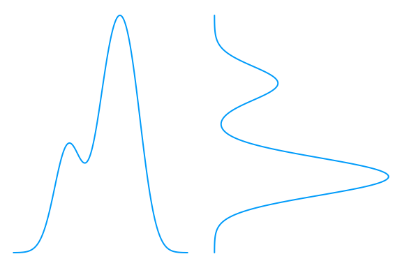
It is important to visualize the trace plots to ensure that the sample didn’t have issues exploring the posterior distribuiton. We are looking for furry caterpillar plots on the left, and Normal-ish plots on the right.

StatsPlots.plot(chain)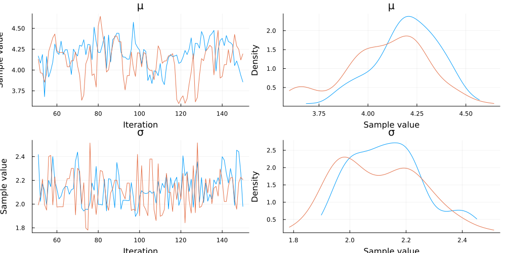

All looks good, now lets dive into a custom visualization of these chains.

Building the MCMC Plot

Since our model only has two parameters, μ and σ, we can visualize the full posterior distribution on a standard two-dimensional plot. I really like how Richard McElreath visualizes Hamiltonian Monte Carlo in his blog. Let’s try and build a plot that looks similar to what he uses to display the different MCMC algorithms.

Posterior Plot

First, we will define a plot of the posterior domain for our model’s parameters. Ignore the legend for now, we will add lines for our chains later on.

# define parameter plot
post_plot = plot(
	xlabel = "μ", 
	ylabel = "σ", 
	legend=:bottom,
	legend_column = -1,
	legendtitle = "Chain",
	legendfontsize = 5,
	legendtitlefontsize = 5
);
post_plot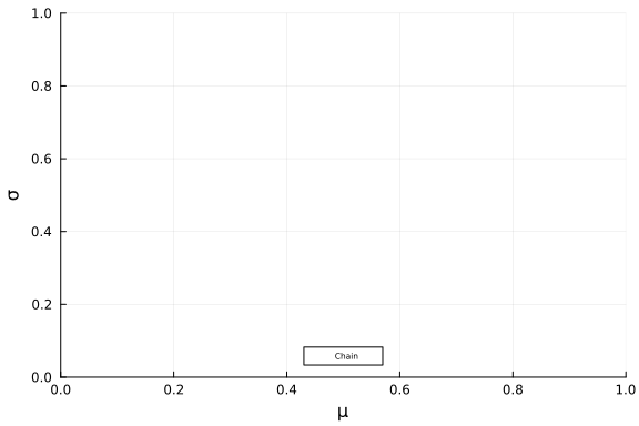

Next we will build a 2D kernel density and add that to our plot. We can do this with the kde function from the KernelDensity.jl library. All we have to do is extract the parameter traces from our chain object and feed them into that function and add it to our plot. With an eye toward plotting sequential draws in a gif, lets first define the draws that we are going to plot. For this example, let’s plot the estimated posterior density on the 2nd draw from each chain.

# define draw number to plot
draw_num = 2

# get the parameters from the chain object
param_trace = chain[["μ", "σ"]][1:draw_num,:,:];

# plot the kernel density
param_dens = kde(Array(param_trace));
plot!(post_plot, param_dens, alpha = 0.25, colorbar = false)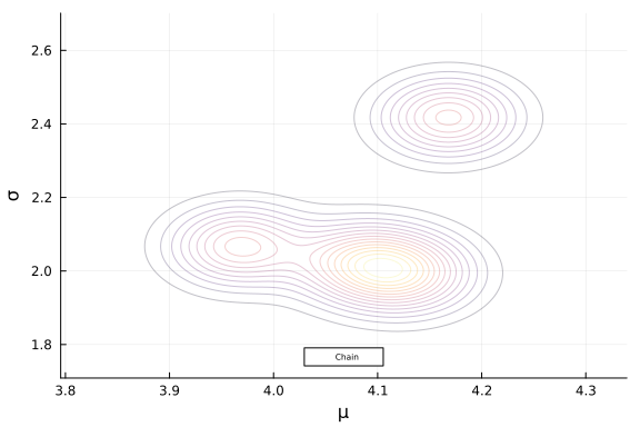

The last element to add to the posterior plot are some lines indicating the path that the sampler is taking through the posterior space. Our param_trace object has three dimensions, draw, parameter, and chain. We can plot individual chains by indexing the third dimension of that object. Lets add the path from the first to second draw for each chain to our plot.

# define sequence step
draw_seq_step = 1
# define draw sequence
draw_seq = ifelse(
	draw_num <= draw_seq_step, 
	draw_num, 
	(draw_num-1):draw_num
)
# plot chains
for chain_num in 1:n_chains
	plot!(
		post_plot,
		param_trace[draw_seq,1,chain_num],
		param_trace[draw_seq,2,chain_num],
		label = "$chain_num",
		alpha = 0.75,
		linewidth = 2,
		arrow = true
	)
end;
post_plot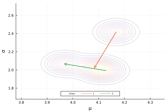

Marginal Density Plots

Now that we have our posterior plot looking good, let’s add marginal density plots to the plot object. we can use the kde function on each of the parameters from the trace. Here I demonstrate how the julia pipe operator |> can be used to iteratively transform your data. We take the paramater trace and transform it to a vector, then pass that through to the kde function. Note, because we want the sigma density to be rotated 90 degrees and displayed on the right side of our posterior plot, we need to pass the density to the x axis and the domain to the y axis in our plot.

# Mu Density
μ_kde = param_trace["μ"].data |> vec |> kde;
μ_density_plot = plot(μ_kde.x, μ_kde.density, legend = false, axis=([],false), linewidth = 2);

# Sigma Density -> need to rotate 90 degrees -> density on x asis
σ_kde = param_trace["σ"] |> vec |> kde;
σ_density_plot = plot(σ_kde.density, σ_kde.x, legend = false, axis=([],false), linewidth = 2);

# Display Mu Density
plot(
	μ_density_plot,
	σ_density_plot
)

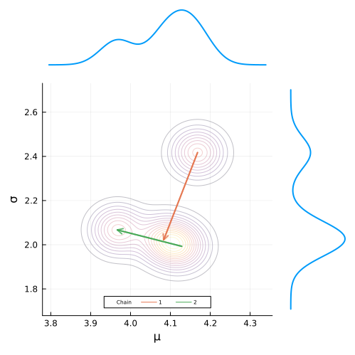
Now we need to add these marginal plots to our posterior plot that we made earlier. To do this, we need to define a custom layout using the @layout macro. We want the μ_density_plot on the top of the post_plot, with on the σ_density_plot on the right. We can use the layout defined below to achieve this, along with using the orientation keyword to indicate the the last plot (the sigma density) needs to oriented vertically. Passing the series of plots into the plot function along with the keyword arguments for layout, orientation, size, etc. produces our final plot.

# Define layout
layout = @layout [a _; b{0.8w,0.8h} c];
# Plot marginal densities and posterior together
plot(
	μ_density_plot,
	post_plot,
	σ_density_plot, 
	layout = layout, 
	link = :both, 
	orientation = [:v :v :h], 
	size = (500, 500), 
	marign = 10Plots.px
)

Creating the Animation

Now that all of the pieces are constructed to build the full plot, we need to define a function that puts it all together. The arguments for our function will include the chain object, as well as the draw number and step size to plot.

function posterior_density_plot(chain::Chains, draw_num::Int, draw_seq_step::Int)

	# Posterior Plot
	post_plot = plot(
		xlabel = "μ", 
		ylabel = "σ", 
		legend=:bottom,
		legend_column = -1,
		legendtitle = "Chain",
		legendfontsize = 5,
		legendtitlefontsize = 5
	)

	# Parameter Trace
	param_trace = chain[["μ", "σ"]][1:draw_num,:,:]

	# Parameter Density
	param_dens = kde(Array(param_trace))
	plot!(post_plot, param_dens, alpha = 0.25, colorbar = false)

	# Chain Steps
	draw_seq = ifelse(
		draw_num <= draw_seq_step, 
		draw_num, 
		(draw_num-1):draw_num
	)
	for chain_num in 1:n_chains
		plot!(
			post_plot,
			param_trace[draw_seq,1,chain_num],
			param_trace[draw_seq,2,chain_num],
			label = "$chain_num",
			alpha = 0.75,
			linewidth = 2,
			arrow = true
		)
	end

	# Mu Density
	μ_kde = param_trace["μ"].data |> vec |> kde;
	μ_density_plot = plot(μ_kde.x, μ_kde.density, legend = false, axis=([],false), linewidth = 2);

	# Sigma Density -> need to rotate 90 degrees
	σ_kde = param_trace["σ"] |> vec |> kde;
	σ_density_plot = plot(σ_kde.density, σ_kde.x, legend = false, axis=([],false), linewidth = 2);

	# Layout
	layout = @layout [a _; b{0.8w,0.8h} c]
	
	# Final Plot
	plot(
		μ_density_plot,
		post_plot,
		σ_density_plot, 
		layout = layout, 
		link = :both, 
		orientation = [:v :v :h], 
		size = (500, 500), 
		marign = 10Plots.px
	)
end;

Defining the animation is super simple. All we have have to do is define a loop that builds the plot frames and add the @animate macro before it’s definition. To build the gif, we simply pass in our animation object along with the desired frames per second and we are good to go!

# Define animation
step_size = 1
anim = @animate for i in (2*step_size):step_size:n_samples
	posterior_density_plot(chain, i, 1)
end

# create folder to save gif
if !isdir("figures")
    mkdir("figures")
end
# pass animation to gif: n frames per second
gif(anim, "figures/mcmc.gif", fps = 7)

And thats all there is to it. In the future I look forward to exploring some of the other cool plotting libraries in Julia.

• 2023 2
• 2020 1