Generalized Additive Models in Julia

Introduction

The motivation to write this post comes from the apparent need for a Julia package to fit Generalized Additive Models, or GAMs. I have found GAMs to be a very useful tool, and both R and Python have good implementations of these types of models in the {mgcv} and pyGAM packages, respectively. As a data scientist looking to learn more about Julia, I thought it would be a worthwhile exercise to unpack GAMs and try to build one in Julia. I am not yet at the competency where I could whip up a mgcv or pyGAM port to Julia, but I wanted to explore how these models are built, and how they could potentially be implemented in Julia.

What are GAMs?

GAMs are tools that allow us to model an outcome variable as the sum of different functions over the input variables. Typically, these functions are smooth function approximations called called splines, but this is not necessary for GAMs. A common approach to building splines is to use basis functions, which allow us to build arbitrarily “wiggly” curves to fit the data. Smoothing splines help avoid over-fitting by regularizing the “wiggliness” of the curves (typically through penalities on the second derivative at the knots).

My Learning Journey

My quest to figure out how to code up these models started at this reply to the Julia Discourse thread linked above. Fitting a mixed effects model using MCMC (aka a Bayesian Hierarchical Model)? That sure caught my attention. So I took a look at the paper referenced in the thread. I quickly realized that if I wanted to build a GAM from scratch, I needed to find a resource that had code. My search then lead me to Tristan Mahr’s FANTASTIC blog post on penalized splines. Serious props to Tristan. His post does an excellent job of building the intuition of how mixed effects models related to penalized smoothing splines. His post references the work of Simon Wood on Generalized Additive Models multiple times, so I figured it would behoove me to go right to the source and pick up a copy of his textbook on the subject. This text is a must read for anyone looking to implement GAMs from scratch. Most of my Julia code is adapted from his R code.

What This Post is

The goal of this post is to demonstrate how to use Julia to fit penalized, smooth splines and additive models to data. It seemed to me that there were sparse resources freely available on the internet that demonstrated how to do this, so I am going to attempt to fill that void. I am not going to go into great detail about what B-Splines are and how to fit them. There are so many great resources out there for that, and I don’t want to re-invent the wheel. I have provided links to many of those resources in the below.

Aknowledgements

This tutorial is heavily inspired by examples from Richard McElreath’s Statistical Rethinking text, specifically his spline examples in Chapter 4. Max Lapan has developed and maintains Julia translations of the Statistical Rethinking codebase. His notes on chapter 4 were very helpful in the development of this tutorial. doggo dot jl has developed a video tutorial demonstrating how to build Bayesian Splines in Julia on their YouTube channel. It provides a really great introduction to the topic with great examples. Simon Wood’s text, Generalized Additive Models: An Introduction with R, is the primary the primary resource I used for learning these topics. The code in this post has been adapted from the R code in the text. Last but certainly not least, I was inspired to learn the concepts in this tutorial by reading Tristan Mahr’s blog post on smoothing splines.

Imports

using Turing # for Bayes
using Random # for reproducibility
using FillArrays # for building models
using MCMCChains # for MCMC sampling
using Distributions # for building model
using DataFrames # for data
using RDatasets # for data
using StatisticalRethinking # for data
using StatsPlots # for plotting
using GLM # for fitting models
using Optim # for optimizing parameters
using BSplines # for splines
using LinearAlgebra # for matrix math

# set seed for reproducibility
Random.seed!(0);

Data

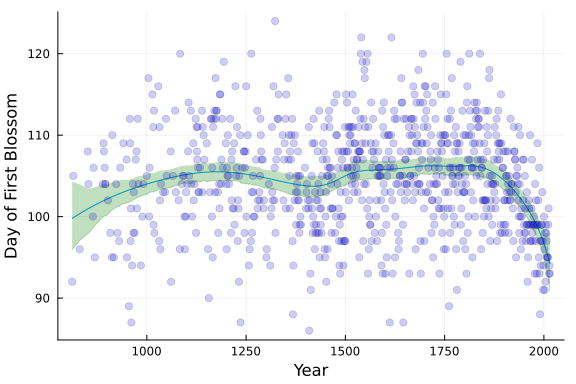
The data set we will be using is the cherry_blossoms dataset, which can be found in Chapter 6 of Statistical Rethinking. We will use the dataset to model the day of year of first blossom for cherry trees in Japan using a univariate smoothing spline (GAM with 1 predictor variable). First, we will load the dataset from the StatisticalRethinking package. We will do some basic data cleaning and look at the first few rows.

# Import the cheery_blossoms dataset.
data = CSV.read(sr_datadir("cherry_blossoms.csv"), DataFrame);

# drop records that have missing day of year values
data = data[(data.doy .!= "NA"),:];

# convert day of year to numeric column
data[!,:doy] = parse.(Float64,data[!,:doy]);

# Show the first five rows of the dataset.
first(data, 5)

5×5 DataFrame Row │ year doy temp temp_upper temp_lower │ Int64 Float64 String7 String7 String7 ─────┼───────────────────────────────────────────────── 1 │ 812 92.0 NA NA NA 2 │ 815 105.0 NA NA NA 3 │ 831 96.0 NA NA NA 4 │ 851 108.0 7.38 12.1 2.66 5 │ 853 104.0 NA NA NA

Our goal is to model the relationship between doy (Day of Year) and year variables. For this exercise, we will center the doy variable to make our spline easier to interpret (more on that later).

# Create x and y variables
x = data.year;
y_mean = mean(data.doy);
y = data.doy .- y_mean;

Let’s plot the relationship between these columns of the data.

# Make a function to make a scatter plot of the raw data
function PlotCherryData(; kwargs...)
    scatter(x,y .+ y_mean,label = "Data"; kwargs...)
    xlabel!("Year")
    ylabel!("Day of First Blossom")
end;

# Plot the data
PlotCherryData()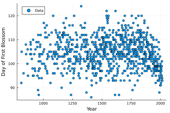

From the plot we can see what appears to be a non-linear relationship between the year and day of first blossom. We will explore this relationship using B-Splines

Building the Basis

There are two parameters we need to define our basis with the BSplines package. These parameters are the number of knots (or breakpoints) and the order of the basis functions. It should be noted that the order of a basis function is equal to the degree plus 1. For example, if we want to use cubic basis functions (degree 3), the order is equal to 3+1=4.

For these data, we will use a cubic spline (order = 4). But how many knots should we choose? In this case, we will use 25 knots. The choice for using a relatively large number of knots will produce a rather “wiggly” fit. In Chapter 4 section 2 of his text, Simon Wood recommends choosing a number of knots that is larger than needed and induce smoothing later.

The following code builds the knots at the quantiles of the independent variable and builds the basis. We can simply call the plot function on the basis object to view the basis functions.

# Parameters to define basis
N_KNOTS = 15;
ORDER = 4; # third degree -> cubic basis

function QuantileBasis(x::AbstractVector, n_knots::Int64, order::Int64)

    # Build a list of the Knots (breakpoints)
    KnotsList = quantile(x, range(0, 1; length=n_knots));

    # Define the Basis Object
    Basis = BSplineBasis(order, KnotsList);

    return Basis
end

Basis = QuantileBasis(x, N_KNOTS, ORDER);

# Plot the Basis Functions
plot(Basis, title = "Basis Functions", legend = false)
xlabel!("Year")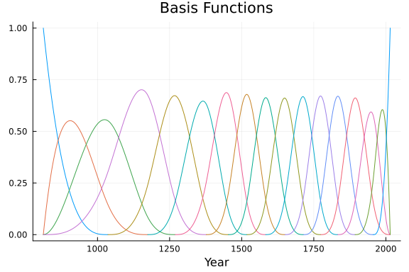

In order to fit our spline regression model, we need to build a design matrix from our basis object. The following code builds our design matrix and plots the matrix using the heatmap function. The plot displayed below outlines the relative weighting that each basis function has on each value of the domain before it is fit.

# Build a Matrix representation of the Basis
function BasisMatrix(Basis::BSplineBasis{Vector{Float64}}, x::AbstractVector)
    splines = vec(
        mapslices(
            x -> Spline(Basis,x), 
            diagm(ones(length(Basis))),
            dims=1
        )
    );
    X = hcat([s.(x) for s in splines]...)
    return X 
end

X = BasisMatrix(Basis, x);

# Plot the basis matrix using the heatmap function
heatmap(X, title = "Basis Design Matrix", yflip = true)
ylabel!("Observation Number")
xlabel!("Basis Function")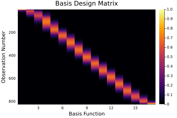

Now that we have a design matrix built from our basis functions, we can fit our model.

Fitting the Spline

The first model we will fit is a simple regression model using OLS. This model won’t have a smoothing penalty applied, and will serve as a comparative baseline for the penalized smoothing splines that we fit later. We can generate our spline function by multiplying the basis design matrix by the regression coefficients, though the BSplines package provides nice functionality with the Spline struct. We can pass in our basis and weights (from OLS) to build the the resulting spline. This struct has a lot of nice methods such as being able to pass in x values and it will evaluate the spline at those values (much like a function would) and it has nice plotting utilities as well.

# Fit model with basic OLS
β_spline = coef(lm(X,y));
# Define Spline Object
Spline_OLS = Spline(Basis, β_spline);

The plots below displays the resulting weighed basis functions, and the resulting spline fit. One thing to note, interpreting this plot is why we centered our doy variable. It makes the relative basis weightings easier to distinguish.

# Plot Weighted Basis 
plot(x, β_spline .* Basis, title = "Weighted Basis Functions", label = "")
plot!(x, Spline_OLS, color = :black, linewidth = 3, label = "Spline Fit", legend = true)
ylabel!("Basis * Weight")
xlabel!("Year")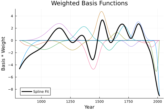

And we can inspect the fit to our data:

# Plot Data and Spline
PlotCherryData(alpha = 0.20)

plot!(
    x,
    # evaluate spline at x and add mean
    Spline_OLS.(x) .+ y_mean, 
    color = :black, 
    linewidth = 3, 
    label = "Spline Fit"
)

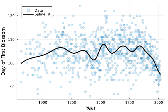
From the plot above, it can be seen the the resulting spline fit to the data is rather “wiggly” and not smooth. It is likely to be overfit. Let’s explore some ways to improve our model’s fit.

Making it Smooth

Smoothness is induced by enforcing a penalty on the second derivative at the knots. The first thing we need to do is build an identity matrix with diagonal the length of the number of basis functions and twice taking the difference of that matrix. To do this, we will first define a general function to take differences of matrices.

# General Function to take differences of Matrices
function diffm(A::AbstractVecOrMat, dims::Int64, differences::Int64)
    out = A
    for i in 1:differences
        out = Base.diff(out, dims=dims)
    end
    return out
end

# Difference Matrix
# Note we take the difference twice.
function DifferenceMatrix(Basis::BSplineBasis{Vector{Float64}})
    D = diffm(
        diagm(0 => ones(length(Basis))),
        1, # matrix dimension
        2  # number of differences
    )
    return D
end

D = DifferenceMatrix(Basis);

The D matrix represents the second derivative at the knots, or breakpoints, of our spline. In order to induce smoothness in our function, we need to apply a penalty to these differences. We can do this by augmenting our objective function to minimize from standard OLS to:

It took me a minute to really grasp what the following code is doing when I first read it. But essentially what we can do is mulitply the lambda parameter by our penalty matrix, D and row-append it to our basis design matrix, X. We then need to append zeros to our outcome vector to make sure the rows are equal between the two. What this allows us to do is use standard OLS to estimate the model coefficients with the lambda penalty applied. Typically when I see penalized regression models the parameters need to be estimated via some optimization algorithm. I just thought it was really cool to the clever use of OLS here.

# Define Penalty
λ = 1.0

# Augment Model Matrix and Outcome Data
function PenaltyMatrix(Basis::BSplineBasis{Vector{Float64}}, λ::Float64, x::AbstractVector, y::AbstractVector)

    X = BasisMatrix(Basis, x) # Basis Matrix
    D = DifferenceMatrix(Basis) # D penalty matrix
    Xp = vcat(X, sqrt(λ)*D) # augment model matrix with penalty
    yp = vcat(y, repeat([0],size(D)[1])) # augment data with penalty

    return Xp, yp
end

Xp, yp = PenaltyMatrix(Basis, λ, x, y);

# Fit Penalized Spline
β_penalized = coef(lm(Xp,yp));
# Define Penalized Spline Object
Spline_penalized = Spline(Basis, β_penalized);

# Plot Data and Spline
PlotCherryData(alpha = 0.20)
plot!(x, Spline_OLS.(x) .+ y_mean, color = :black, linewidth = 3, label = "Basic Spline")
plot!(x, Spline_penalized.(x) .+ y_mean, color = :red, linewidth = 3, label = "Penalized Spline")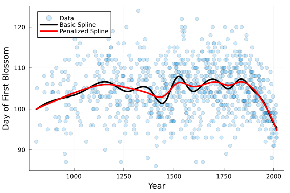

From the plot above we can see that the red penalized spline with λ = 1 is smoother than the black basic spline fit. But how can we determine what the optimal value for lambda should be?

Finding Optimal Penalty

One obvious approach to finding the optimal penalty is to use cross validation. In his text, Wood outlines a method of using Generalized Cross Validation to determine the optimal penalty. I can’t say that I have an intuitive understanding of this method, but it seems fairly similar to leave one out cross validation. I was able to adapt Wood’s R code from his text to Julia. The code for these functions are below, and the optimal lambda value for our example is calculated to be around 72.

# Function to calculate GCV for given penalty
function GCV(param::AbstractVector, Basis::BSplineBasis{Vector{Float64}}, x::AbstractVector, y::AbstractVector)
    n = length(Basis.breakpoints)
    Xp, yp = PenaltyMatrix(Basis, param[1], x, y)
    β = coef(lm(Xp,yp))
    H = Xp*inv(Xp'Xp)Xp' # hat matrix
    trF = sum(diag(H)[1:n])
    y_hat = Xp*β
    rss = sum((yp-y_hat)[1:n].^2) ## residual SS
    gcv = n*rss/(n-trF)^2
    return gcv
end

# Function that Optimized Lambda based on GCV
function OptimizeGCVLambda(Basis::BSplineBasis{Vector{Float64}}, x::AbstractVector, y::AbstractVector)

    # optimization bounds     
    lower = [0]
    upper = [Inf]
    initial_lambda = [1.0]

    # Run Optimization
    inner_optimizer = GradientDescent()
    res = Optim.optimize(
        lambda -> GCV(lambda, Basis, x, y), 
        lower, upper, initial_lambda, 
        Fminbox(inner_optimizer)
    )
    return Optim.minimizer(res)[1]
end

λ_opt = OptimizeGCVLambda(Basis, x, y);

Now that we have obtained an optimal value for lambda, we can build the penalized design matrix and fit our spline.

Xp_opt, yp_opt = PenaltyMatrix(Basis, λ_opt, x, y);

# Fit Optimized Spline
β_opt = coef(lm(Xp_opt,yp_opt));
# Define Optimized Spline Object
Spline_opt = Spline(Basis, β_opt);

PlotCherryData(alpha=0.2)
plot!(x, Spline_OLS.(x) .+ y_mean, color = :black, linewidth = 3, label = "Basic Spline")
plot!(x, Spline_penalized.(x) .+ y_mean, color = :red, linewidth = 3, label = "Spline: λ = 1")
plot!(x, Spline_opt.(x) .+ y_mean, color = :blue, linewidth = 3, label = "Spline: λ = $(round(λ_opt,digits=3))")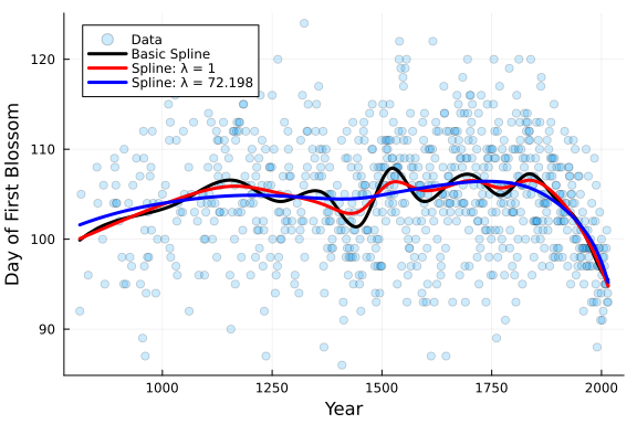

It is clear that the blue spline, with penalty of λ = 72.198 is far smoother than the other splines we fit. That is exactly what we were looking for, but this is not the only avenue to obtain this result.

Using a Bayesian Hierarchical Approach

Now for the fun stuff. In order to use a Bayesian approach, we need to re-parameterize our model. Wood goes into detail on the theory of this parameterization on pages 173-174 of his text. The procedure involves some pretty low level linear algebra. To be truthful, I do not have a good intuition of what the matrix algebra is doing for us here. But I was able to figure out how to translate the R code into Julia.

For those looking for a more detailed explanation of this math, I will have to point you to Wood’s text.

One thing to note on terminology, Bayesian Hierarchical are sometimes called “Random Effects” models, and models with no established hierarchy are referred to as “Fixed Effects” models. Models with hierarchical and non-hierarchical variables are called “Mixed Effect” models (having both random and fixed variables). For the example below, I will adopt the terminology of “random” and “fixed” effects.

From this Julia code, the resulting X_fe matrix represents the fixed effects matrix and Z_re represents the random effect matrix.

# Function to build the Mixed Effect Matricies
function MixedEffectMatrix(Basis::BSplineBasis{Vector{Float64}}, x::AbstractVector)

    # Build Basis Matrix
    X = BasisMatrix(Basis, x)

    # Build difference Matrix
    D = DifferenceMatrix(Basis)

    ## Reparameterization
    D_pls = vcat(zeros(2,length(Basis)), D);
    D_pls[diagind(D_pls)] .= 1;
    XSD = (UpperTriangular(D_pls') \ X')';

    # Split to Fixed and Random Effects
    X_fe = XSD[:, 1:2]; # Fixed
    Z_re = XSD[:, 3:end]; # Random

    return X_fe, Z_re
end

X_fe, Z_re = MixedEffectMatrix(Basis, x);

We can now define our Turing model to fit the hierarchical smoothing spline model. This model function accepts the following arguments:

• X_fe is the fixed effect matrix;
• Z_re is the random effect matrix;
• y is the element we want to predict;
• μ_int is the center of the intercept prior;
• σ_prior is the standard deviation of coefficient priors;
• err_prior defines the exponential prior on likelihood error;
• re_prior defines the exponential prior on random effect variance.

# Define Turing model
@model function SmoothSplineModel(X_fe, Z_re, y, μ_int, σ_prior, err_prior, re_prior)

    ## Priors 
    # Intercept
    α ~ Normal(μ_int, σ_prior)

    # Fixed Effects
    B ~ MvNormal(repeat([0],2), σ_prior)
    
    # Random Effects
    μ_b ~ Normal(0, σ_prior)
    σ_b ~ Exponential(re_prior)
    b ~ filldist(Normal(μ_b, σ_b), size(Z_re)[2])
    
    # error
    σ ~ Exponential(err_prior)

    ## Determined Variables
    μ = α .+ X_fe * B + Z_re * b
    
    ## Likelihood
    y ~ MvNormal(μ, σ)
end;

We will use MCMC to perform inference. The following code will use the No U-turn (NUTS) sampler to draw 1000 samples from the posterior. Typically it is advised to run multiple chains, see the Turing docs, but for this demo we will use just a single chain. Turing has a lot of neat features, such as the ability to simply call summarystats(chain) to assess model convergence.

One thing to note: Since we are fitting the y-intercept variable α in this model, there is no need to use the centered version of y here.

# Define Model Function
## Note adding y_mean back to y
spline_mod = SmoothSplineModel(X_fe, Z_re, y .+ y_mean, 100, 10, 5, 5);

# MCMC Sampling
chain_smooth = sample(spline_mod, NUTS(), 1_000);

# Summary
summarystats(chain_smooth)

Summary Statistics parameters mean std naive_se mcse ess rhat ⋯ Symbol Float64 Float64 Float64 Float64 Float64 Float64 ⋯

       α   100.9578    5.6333     0.1781    0.2900   371.9183    0.9990
⋯
    B[1]    -1.1778    5.6998     0.1802    0.2881   356.6087    0.9991
⋯
    B[2]     1.2111    5.5418     0.1752    0.2848   369.8150    0.9990
⋯
     μ_b    -0.3800    0.6335     0.0200    0.0211   702.2543    0.9991
⋯
     σ_b     2.2553    1.1081     0.0350    0.1023    76.1735    1.0261
⋯
    b[1]    -0.1599    2.1407     0.0677    0.0843   507.3550    0.9996
⋯
    b[2]    -0.8512    1.8899     0.0598    0.0674   527.4515    1.0007
⋯
    b[3]    -2.0182    1.6583     0.0524    0.0862   336.3577    0.9990
⋯
    b[4]    -0.5716    1.5628     0.0494    0.0594   800.0749    0.9997
⋯
    b[5]     0.7625    1.6226     0.0513    0.0569   890.2162    1.0007
⋯
    b[6]     2.7054    2.2498     0.0711    0.1585   135.8350    1.0154
⋯
    b[7]    -2.3017    2.4691     0.0781    0.1916   117.8017    1.0097
⋯
    b[8]     0.3076    1.7181     0.0543    0.0777   375.2523    0.9993
⋯
    b[9]     0.1552    1.6209     0.0513    0.0622   605.8256    1.0024
⋯
   b[10]    -0.7186    1.6908     0.0535    0.0960   281.5948    1.0052
⋯
   b[11]     0.7085    1.8439     0.0583    0.1153   205.5236    1.0069
⋯
   b[12]    -1.8647    1.7745     0.0561    0.0797   554.2207    1.0004
⋯
  ⋮           ⋮          ⋮         ⋮          ⋮         ⋮          ⋮   
⋱
                                                 1 column and 4 rows om itted

We can then take the mean of the posterior for each parameter and build the spline predictions for each observation to compare with our previous models.

# Get posterior draws for relevant parameters
post_smooth = get(chain_smooth, [:α, :B, :b]);

# Compute Predictions
pred_smooth = [post_smooth[:α]...]' .+ X_fe * hcat(post_smooth[:B]...)' .+ Z_re * hcat(post_smooth[:b]...)';

The following plot compares the original spline model to the smoothing spline model that we just fit. As we can see, the smoothing spline fit looks far smoother despite having the exact same number of knots and basis functions as the original model.

# Plot Data and Splines
PlotCherryData(alpha=0.2)
plot!(x, Spline_opt.(x) .+ y_mean, color = :blue, linewidth = 3, label = "Spline: λ = $(round(λ_opt,digits=3))")
plot!(x, mean(pred_smooth;dims=2), color = :green, linewidth = 3, label = "Spline: Bayes")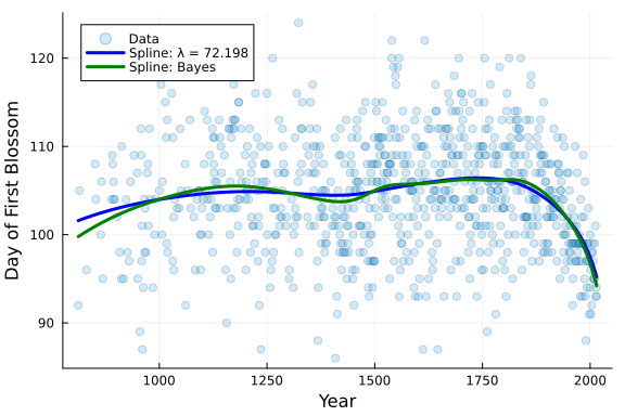

Since our outcomes are so similar, what are we getting using the Bayesian model over optimizing the λ penalty? Well, one benefit is that we can use the model posterior to build the posterior predictive distribution for the outcome. This gives us a probability distribution over the outcome, which can be useful.

This is a way to take advantage of the full uncertainty quantification that a Bayes model gives us. The following Julia code demonstrates how we can leverage the full posterior for predictions by building a partial dependence plot.

function PartialDepPlot(x,pred)

    # Sort Data
    x_order = sortperm(x)
    x = x[x_order]
    pred = pred[x_order,:]

    # Build HDI
    hdi = mapslices(x -> hpdi(x,alpha=0.05), pred; dims=2);

    # Build Partial Dependence Plot
    plt = plot(x, mean(pred;dims=2));
    plot!(
        plt,
        x, hdi[:,1], 
        fillrange = hdi[:,2],
        color = :green, fillcolor = :green,
        alpha = 0.25, fillalpha = 0.25,
        legend = false
    );
    return plt;
end

# Plot the HDI
PartialDepPlot(x, pred_smooth)
scatter!(
    x, y .+ y_mean,
    color=:blue,
    xlabel="Year",
    ylabel="Day of First Blossom",
    legend=false,
    alpha=0.2
)

More Variables: Building an Additive Model

Now that we have Julia code capable of building univariate smoothing splines, let’s try our hand at building an additive model with two predictor variables. This example uses the trees dataset from the RDatasets package. The data set has three variables, tree volume, girth, and height. We will build an additive model that builds smooth splines over Girth and Height and predicts the tree Volume. This is the same data set that Simon Wood uses in section 4.3 of his text. But this example is going to differ in approach, it will use the Bayesian approach for our GAM model.

First let’s load the data and plot the relationships.

# Load Data
trees = dataset("datasets", "trees");

# Define Variables
y = trees.Volume;
x1 = trees.Girth;
x2 = trees.Height;

# Plot the Data
plot(
    scatter(x1,y,legend=false,xlabel = "Tree Girth"),
    scatter(x2,y,legend=false,xlabel = "Tree Height"),
    ylabel = "Tree Volume"
)

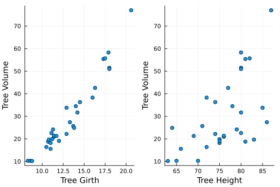
The relationships look like they could be fairly well modeled with a standard linear model. We will see how the smoothing splines approximate these relationships.

The following code loads the data set and performs the data-preprocessing steps from above.

# Build Basis Functions
Basis1 = QuantileBasis(x1, 10, 4);
Basis2 = QuantileBasis(x2, 10, 4);

# Build Mixed Effects Matrices
X_fe_1, Z_re_1 = MixedEffectMatrix(Basis1, x1);
X_fe_2, Z_re_2 = MixedEffectMatrix(Basis2, x2);

# Organize Matrices in Vectors
X_fe = [X_fe_1, X_fe_2];
Z_re = [Z_re_1, Z_re_2];

Next, we will define a Turing Model similar to the one above, but this model now builds two smoothing splines instead of one. I am certain there is a more elegant “Julian” way to build this, but for now the verbose approach will suffice.

# Define Additive Model that uses two splines
@model function AdditiveModel(X_fe, Z_re, y, μ_int, σ_prior, err_prior, re_prior)

    ## Priors 
    # Intercept
    α ~ Normal(μ_int, σ_prior)

    # Fixed Effects
    ## Variable 1
    B1 ~ MvNormal(repeat([0],2), σ_prior)
    ## Variable 2
    B2 ~ MvNormal(repeat([0],2), σ_prior)
    
    # Random Effects
    ## Variable 1
    μ_b1 ~ Normal(0, σ_prior)
    σ_b1 ~ Exponential(re_prior)
    b1 ~ filldist(Normal(μ_b1, σ_b1), size(Z_re[1])[2])
    ## Variable 2
    μ_b2 ~ Normal(0, σ_prior)
    σ_b2 ~ Exponential(re_prior)
    b2 ~ filldist(Normal(μ_b2, σ_b2), size(Z_re[2])[2])
    
    # error
    σ ~ Exponential(err_prior)

    ## Determined Variables
    μ = α .+ X_fe[1] * B1 + X_fe[2] * B2 + Z_re[1] * b1 + Z_re[2] * b2
    
    ## Likelihood
    y ~ MvNormal(μ, σ)
end;

Next, we will instantiate our model, run MCMC to assess parameter posterior values, and build predictions.

# Define Model Function
add_mod = AdditiveModel(X_fe, Z_re, y, 30, 5, 1, 1);

# MCMC Chain
chain_add = sample(add_mod, NUTS(), 1_000);

# Get Posterior Draws
post_add = get(chain_add, [:α, :B1, :B2, :b1, :b2]);

# Compute Predictions
## Girth
pred_add_1 = X_fe_1 * hcat(post_add[:B1]...)' +  Z_re_1 * hcat(post_add[:b1]...)';
## Height
pred_add_2 = X_fe_2 * hcat(post_add[:B2]...)' +  Z_re_2 * hcat(post_add[:b2]...)';
## Volume
pred_add = [post_add[:α]...]' .+ (pred_add_1 + pred_add_2);

And inspect our partial dependence plots.

GirthPlot = PartialDepPlot(x1, pred_add_1);
xlabel!(GirthPlot, "Tree Girth");
HeightPlot = PartialDepPlot(x2, pred_add_2);
xlabel!(HeightPlot, "Tree Height");
plot(GirthPlot, HeightPlot, plot_title = "Partial Dependence Plots")
ylabel!("Tree Volume")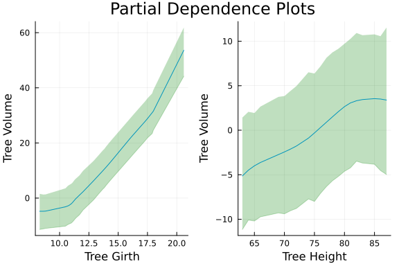

Lastly, we can observe the relationship between actual and predicted tree volume.

# Compute R Squared
RSqrd = cor(y, mean(pred_add;dims=2))[1,1]^2

# Plot Actual v Predictions
scatter(
    y, mean(pred_add;dims=2), 
    legend = false,
    plot_title = "Predicted Volume v Actual Volume"
);
annotate!((20, 60, "R2: $(round(RSqrd,digits=3))"));
xlabel!("Tree Volume");
ylabel!("Predicted Volume")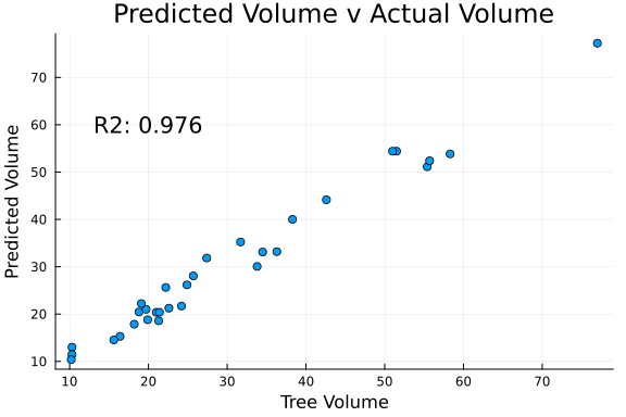

Obviously we would need to hold out some data to properly assess model accuracy.

The objective of the post was to build a GAM in Julia “from scratch”. I am fairly happy with the results, but there is certainly room for improvement. If you made it this far, I want to thank you for your interest in this topic. I hope you found my post on smoothing splines useful.

• 2023 2
• 2020 1